Protein VAEs

Life, in essence, is a dizzying chemical dance choreographed by proteins. It's so incomprehensibly complex that most of its patterns still elude us. But there are methods in the madness – and finding them is the key to fighting disease and reducing suffering. Here is one:

Binding pockets are "hands" that proteins use to act on their surroundings: speed something up, break something down, guide something along.

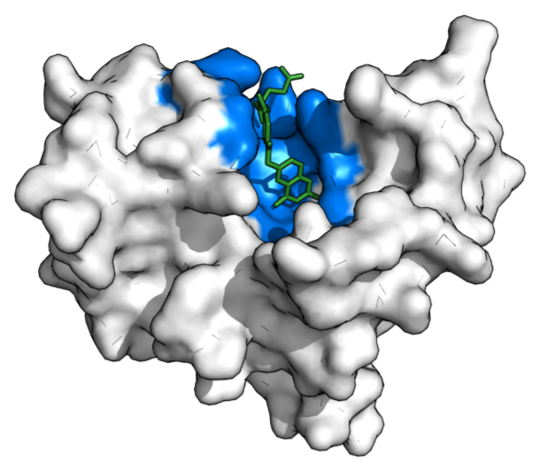
Image from https://en.wikipedia.org/wiki/Binding_site.

Over billions of years, evolution introduces random mutations into every protein. There is a pattern: the binding pockets almost never change. This is perhaps unsurprising: they are the parts that actually do the work! Spoons come in different shapes and sizes, but the part that scoops never changes.

That's why the evolutionary history of a protein, in the form of a Multiple Sequence Alignment (MSA), holds such important clues to the protein's structure and function – its role in this elusive dance. Positions that correlate in the MSA tend to have some important relationship with each other, e.g. direct contact in the folded structure.

A possible explanation: these correlated positions form a binding pocket with some important function. A willy-nilly mutation to one position disrupts the whole binding pocket and renders the protein useless. Throughout evolution, poor organisms that carried that mutation didn't survive and are therefore absent from the MSA.

In a previous post, we talked about ways of teasing out such information from MSAs using pair-wise models that account for every possible pair of positions. But what about the interactions between 3 positions? Or even more? Binding pockets, after all, are made up of many positions. Unfortunately, accounting for all the possible combinations in this way is computationally impossible.

This post is about a solution to this problem of accounting for these far-too-numerous combinations – using a tool from machine learning called variational autoencoders (VAEs). If you're new to VAEs, check out this deep dive!

An introduction to variational autoencoders

Predicting protein function using deep generative models. Latent variable models, reconstruction, variational autoencoders (VAEs), Bayesian inference, evidence lower bound (ELBO).

https://liambai.com/variational-autoencoder

The idea

Latent variables

Imagine some vector $\mathbf{z}$, a latent variable, that distills all the information in the MSA. All the interactions: pairwise, any 3 positions, any 4... Knowing $\mathbf{z}$, we'd have a pretty good idea about the important characteristics of our protein.

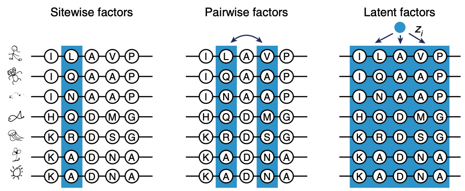
Applying latent variable models like VAEs to MSAs. Figure from 1.

We can view $\mathbf{z}$ as a form of data compression: piles of sequences in our MSA $\rightarrow$ one small vector . Here's the key insight of VAEs: we might not actually know how to most effectively do this compression is; let's ask neural networks to figure it out. We call the neural network that creates $\mathbf{z}$ an encoder.

VAEs in a nutshell

Given a protein sequence, let's ask the encoder: can you capture (in $\mathbf{z}$) its salient features? For example, which positions work together to form a binding pocket? There are 2 rules:

1. No BS. You have to actually distill something meaningful about the input sequence. As a test, a neural network (called a decoder) needs to be able to tell from $\mathbf{z}$ what the input sequence was, reasonably well. This rule is called reconstruction.

2. No rote memorization. If you merely memorize the input sequence, you'll be great at reconstruction but you'll be stumped by sequences you've never seen before. This rule is called regularization.

The tension between these two rules – and the need to balance them – is a common theme in machine learning. For VAEs, they define the two terms of the loss function we use while training.

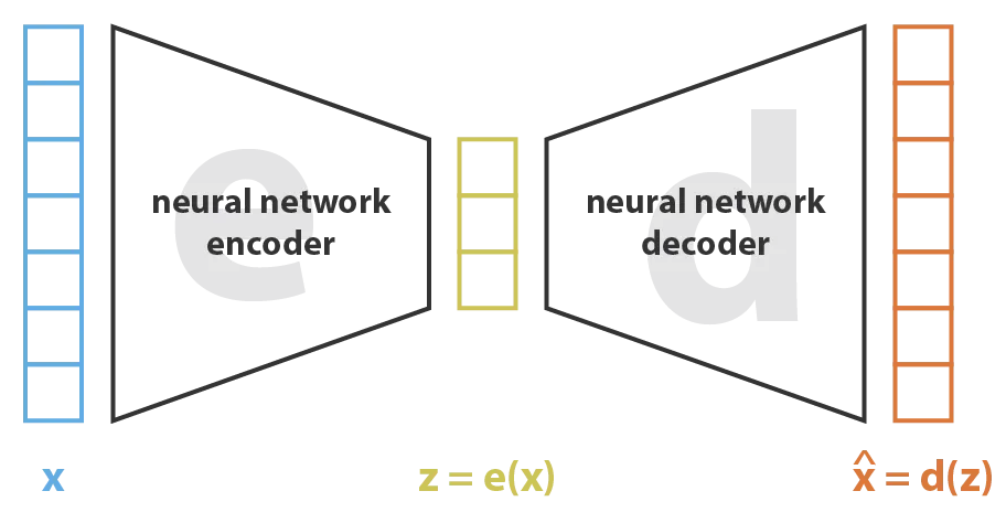
Variational autoencoders are a type of encoder-decoder model. Figure from this blog post.

The model

Intuition aside, what does the model actually look like? What are its inputs and outputs? Concretely, our model is just a function that takes a protein sequence, say ILAVP, and spits out a probability, $p(\mathrm{ILAVP})$:

With training, we want this probability to approximate how likely it is for ILAVP to be a functional variant of our protein.

This probability is the collaborative work of the encoder and the decoder, which are trained together.

An accurate model like this is powerful. It enables us to make predictions about protein variants we've never seen before – including ones associated with disease – or even engineer new ones with properties we want.

Training & inference

Training our model looks something like this:

1. Take an input sequence, say ILAVP, from the MSA.
2. Pass it through encoder and decoder: $\mathrm{ILAVP} \xrightarrow{encoder} \mathbf{z} \xrightarrow{decoder} p(\mathrm{ILAVP}).$
3. Compute the loss function.
4. Use gradient descent to update the encoder and decoder parameters (purple arrow).
5. Repeat.

After going through each sequence in the MSA, our model should have a decent idea of what it's like to be this protein!

Now, when given an unknown input sequence, we can pass it through the VAE in the same way and produce an informed probability for the input sequence (green arrow).

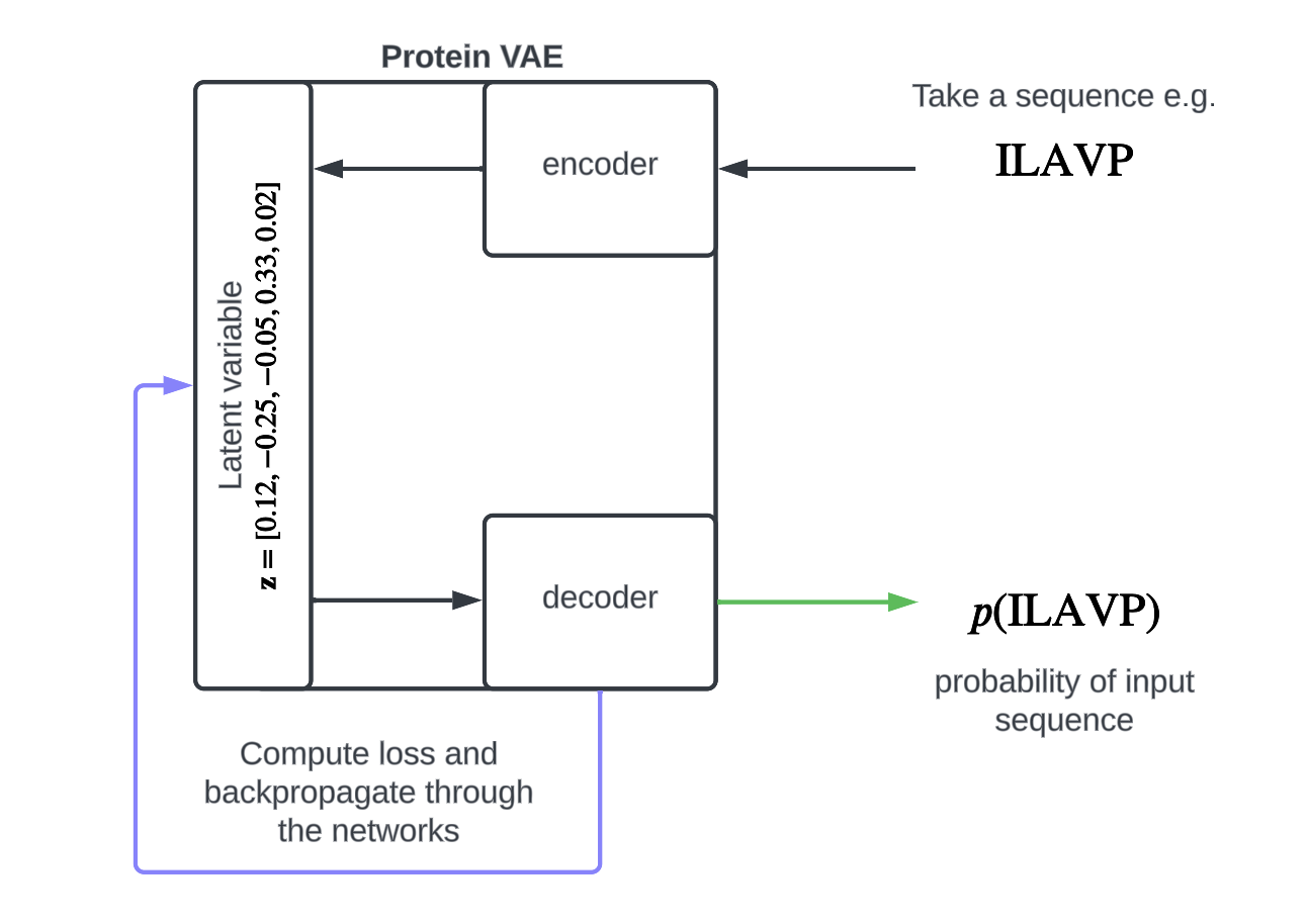
Once trained, we can think of our model's predictions, e.g. $p(\mathrm{ILAVP})$, as a measure of fitness:

• $p(\mathrm{ILAVP})$ is low $\rightarrow$ ILAVP is garbage and probably won't even fold into a working protein.
• $p(\mathrm{ILAVP})$ is high $\rightarrow$ ILAVP fits right in with the natural variants of this protein – and probably works great.

Now, let's put our model to use.

VAEs at work

Predicting disease variants

The explosion in DNA sequencing technology in the last decade came with a conundrum: the enormous amounts of sequence data we unlocked far exceeds our ability to understand them.

For example, genomAD is a massive database of sequence data. If we look at all the human protein variants in genomAD and ask: for how many of these do we know their disease consequences? The answer is: a mere 2%. This means that:

1. We are deeply ignorant about the proteins in our bodies and how their malfunctions cause disease.

2. Unsupervised approaches like VAEs that don't require training on known disease outcomes can make a big impact.

Imagine an in-silico tool that can look at every of possible variant of a protein and make a prediction about its consequence: producing a heatmap like this, where red tiles flag potentially pathogenic variants to watch out for.

EVE (Evolutionary model for Variant Effect) is a protein VAE. Here is a heatmap of it's predictions on the SCN1B protein. Blue = beneficial; red = pathogenic.

A map like this, if dependable, is so valuable precisely because of our lack of experimental data. It enables physicians to make clinical decisions tailored to a specific patient's biology – a growing field known as precision medicine.

Computing pathogenicity scores

How can we compute a map like that? Given a natural sequence (called wild-type) and a mutant sequence, the log ratio

measures the improvement of the mutant over the wild-type .

• If our model favors the mutant over the wild-type $\rightarrow$ $p(\text{mutant}) > p(\text{wild-type})$ $\rightarrow$ positive log ratio $\rightarrow$ the mutation is likely beneficial.

• If our model favors the wild-type over the mutant $\rightarrow$ $p(\text{wild-type}) > p(\text{mutant})$ $\rightarrow$ negative log ratio $\rightarrow$ the mutation is likely harmful.

We can create our map by simply computing this log ratio, a measure of pathogenicity, for every possible mutation at each position.

Evaluating our predictions

How do our model's prediction match up against actual experimental outcomes? On benchmark datasets, the VAE-based EVE did better than all previous models.

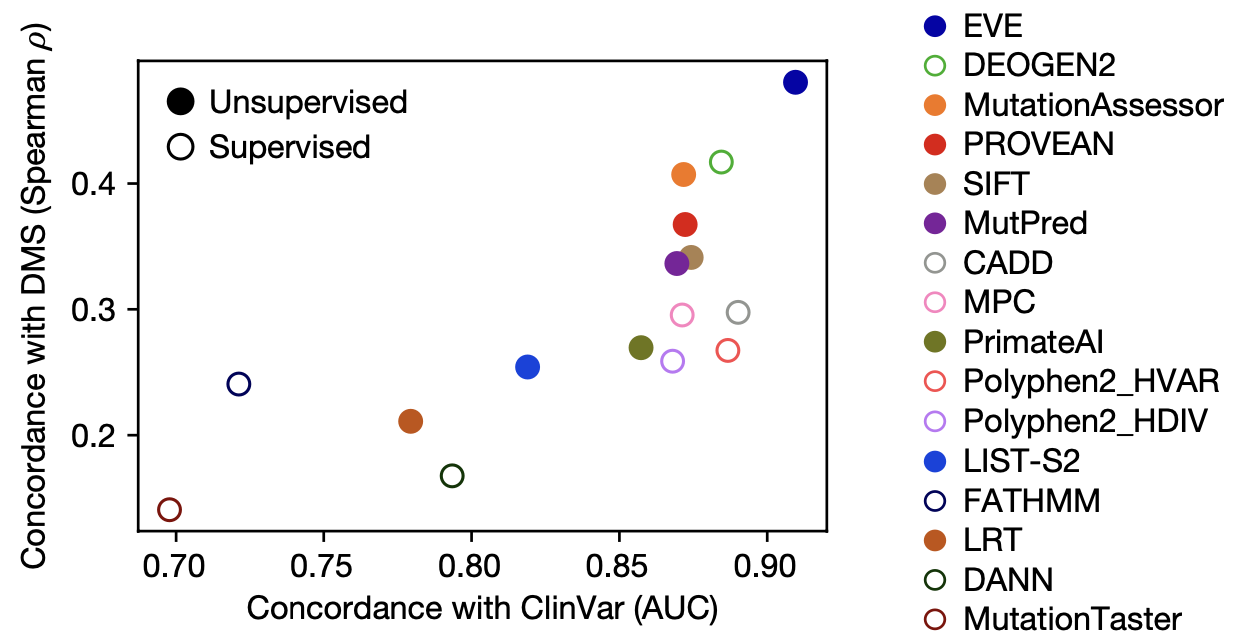
EVE outperforms other computational methods of variant effect prediction in concordance with two experimental dataset. On the x-axis, ClinVar is a database of mutation effects in proteins important to human health. On the y-axis, Deep Mutational Scanning (DMS) is an experimental method for screening a large set of variants for a specific function. Figure from 2.

Remarkably, EVE acquired such strong predictive power despite being completely unsupervised! Having never seen any labeled data of mutation effects, it learned entirely through studying the evolutionary sequences in the protein's family.

Predicting viral antibody escape

A costly challenge during the COVID pandemic was the constant emergence of viral variants that evolved to escape our immune system, a phenomenon known as antibody escape .

Could we have flagged these dangerous variants ahead of their breakout? Such early warnings would have won life-saving time for vaccine development.

VAEs to the rescue: EVEScape is a tool that combines EVE's mutation fitness predictions with biophysical data to achieve accurate predictions on antibody escape.

Given a mutation, EVEScape leverages the VAE-based EVE's predictions in conjunction with biophysical information to produce a score, $P(\text{mutation escapes immunity})$. A high score is an alarm call for a potentially dangerous variant. Figure from 3.

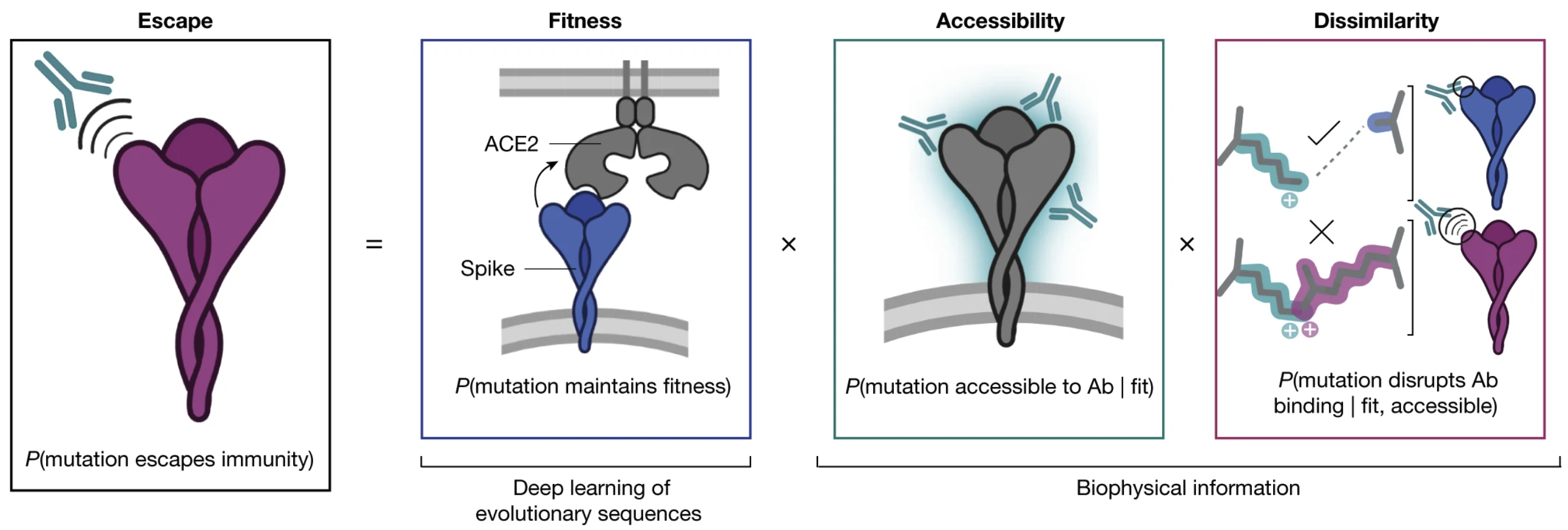
Had we employed EVEScape early in the pandemic – which only requires information available at the time – we would have been alerted of harmful variants months before their breakout.

Figure from 3.

Applicable also to other viruses such influenza and HIV, machine learning tools like EVEScape will play a big role in public health decision-making and pandemic preparedness in the future.

The power of latent variables

VAEs capture complex interactions

Compared to the independent and pair-wise statistical models from a previous post, VAEs are much more accurate.

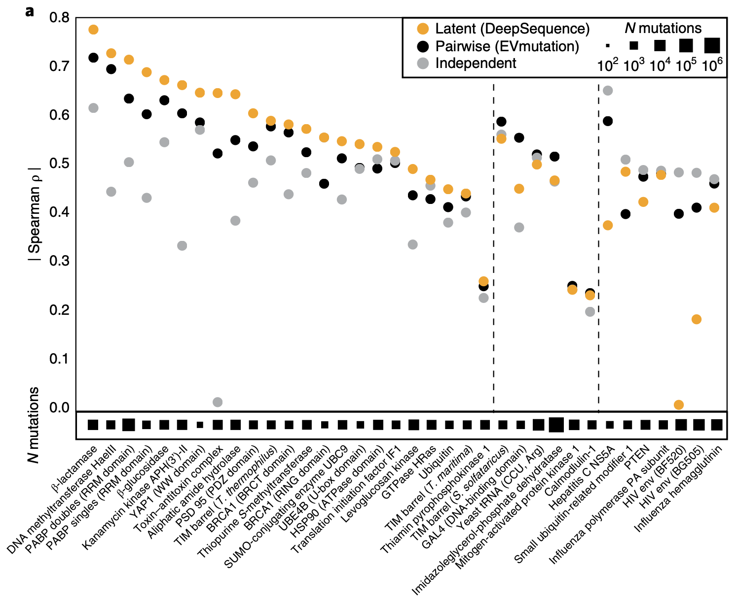
Comparing DeepSequence, a VAE, to statistical models on variant effect prediction, evaluated on Deep Mutational Scanning (DMS) datasets that contain the observed fitness of a many variants. Let's rank them from best to worse. Meanwhile, we can ask our models to make predictions about each variant and produce a ranking. We want these two rankings to be similar! How similar they are is measured by Spearman's rank correlation and plotted on the y-axis. Black dots are results of pair-wise models; grey dots are results of position-wise models. Figure from 1.

The positions at which their accuracy improved the most are ones that cooperate with several other positions – e.g. in forming binding pockets! The latent variable model is better at capturing these complex, multi-position interactions.

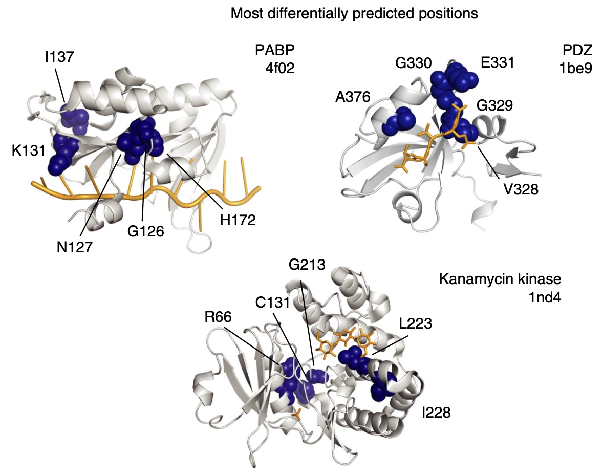
For each protein, the top 5 positions at which DeepSequence showed the most improvement over the independent model. They tend to collaboratively constitute a key functional component of the protein, e.g. a binding pocket. Figure from 1.

Here's one way to look at these results. MSAs contain a wealth of information, some of which we can understand through simple statistics: position-wise frequencies, pair-wise frequencies, etc. Those models are interpretable but limiting – they fail at teasing out more complex, higher-order signals.

Enter neural networks, which are much better than us at recognizing those signals hidden in MSAs. They known where to look, what to look at – beyond our simple statistics. This comes at the cost of interpretability.

Conceding our ignorance

Computer vision had a similar Eureka moment. When processing an image – in the gory details of its complex pixels arrangements – a first step is to extract some salients features we can work with, e.g. vertical edges. To do this, we use a matrix called a filter (also known as a kernel).

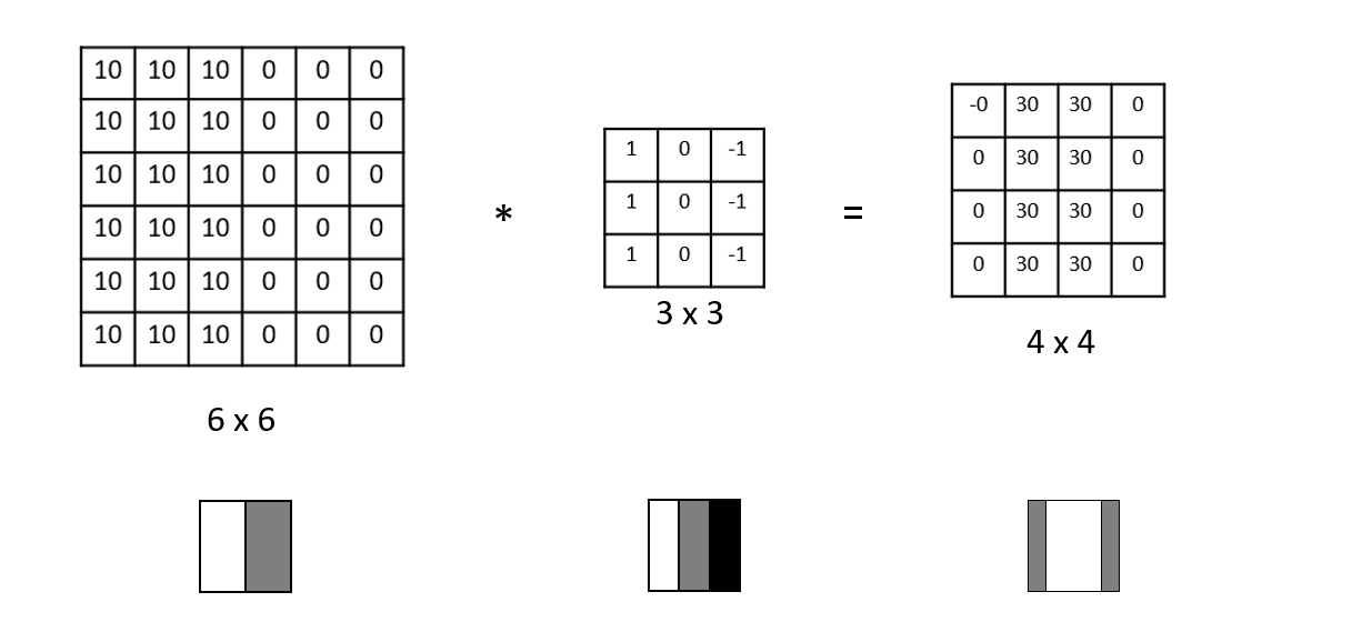
For example, this 3x3 matrix encodes what it means to be a vertical edge. Multiplying it element-wise with a patch in our image and summing the results tells us how much that patch resembles a vertical edge. Repeating this for each patch, we get a convolution, the basis of Convolutional Neural Networks (CNNs).

For a while, researchers came up with carefully crafted filters, each with its mathematical justifications. For example, there was the Sobel filter, the Scharr filter...

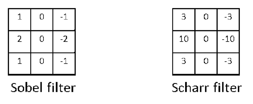
But what if we don't really know what the best filter should look like? In fact, we probably don't even know what to look for: vertical edges, horizontal edges, 45% edges, something else entirely... So why not leave these as parameters to be learned by neural networks? That's the key insight of Yann LeCun in his early work on character recognition, inspiring a revolution in computer vision.

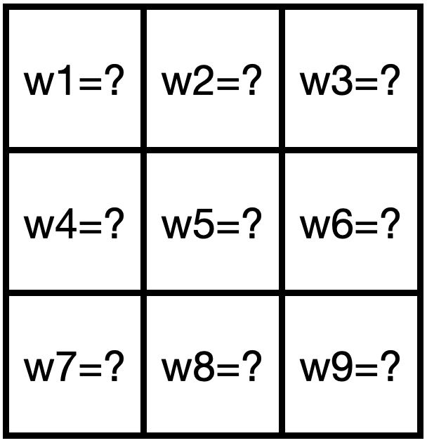
A learned filter, where the values of the matrix are weights to be learned by the neural network.

We are conceding our ignorance and yielding control: we don't know what's best, but neural nets, trained end-to-end, might. This act of humility has won out time and again. To excel at protein structure prediction, AlphaFold similarly limited opinionated processing on MSAs and operated on raw sequences instead. Our protein VAEs do the same thing here.

References

Riesselman, A.J. et al. Deep generative models of genetic variation capture the effects of mutations. Nat Methods 15, 816–822 (2018).
Frazer, J. et al. Disease variant prediction with deep generative models of evolutionary data. Nature 599, 91–95 (2021).
Thadani, N.N. et al. Learning from prepandemic data to forecast viral escape. Nature 622, 818–825 (2023).
- Typically: z is a vector of ~30 numbers, each protein sequence are a few hundred characters long, MSAs have >1000 sequences.
- This is equivalent to the energy-based equations we derived here for the a pair-wise model.
- Antibodies are natural fighters in our bodies that fend off viruses. Vaccines work by amplifying them.